Machine Learning for Signal Propagation
I was interested in exploring the feasibility of performing signal propagation modeling on a mobile device. While signal propagation modeling is not a new field (it dates back to the 1950’s), the concept of doing so accurately and in a computationally-constrained environment is fairly novel. Most simulation packages are firmly focused on accuracy above all else and can only be run in a dedicated desktop environment. I was interested in developing an application that could do the following:
-
Perform calculations on a mobile device in a reasonable timeframe
-
Handle a range of transmission frequencies and physical terrain
-
Balance accuracy and runtime
This project would be considered a simple example of Surrogate Modeling. Surrogate Modeling uses Machine Learning (ML) and other techniques to approximate computationally expensive simulations / calculations with simpler / faster algorithms.
The GitHub repository corresponding to this project can be found here: https://github.com/connor-passe/Sig-Map
Baseline Comparison:
As mentioned above, the two main features of the algorithm I care about are runtime and accuracy. Intuitively, there is a fundamental trade-off between the two. The more compute dedicated to modeling, the better the prediction and the corresponding accuracy, at a cost of higher runtime. To provide context during development, an algorithm was needed to serve as a baseline.
The algorithm I selected for baselining was Free-Space Path Loss (FSPL). Free-Space Path Loss refers to the loss in signal energy as a signal passes through a direct, obstacle-free path. This is a classic inverse square law equation, where intensity drops off proportional to the inverse square of distance. While proprietary commercial models have higher performance, FSPL provides a simple, ball-park baseline for comparison purposes.
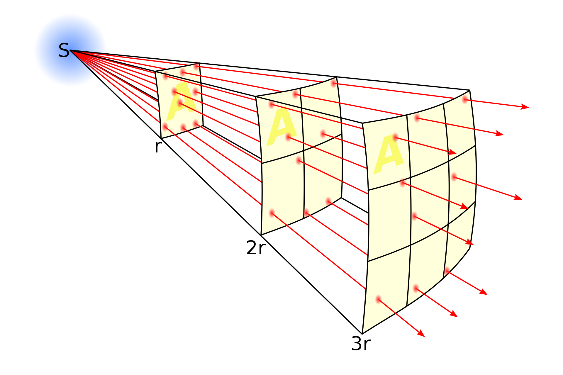
Visual Intuition Behind FSPL
The FSPL algorithm is an O(n) algorithm, with n corresponding to the number of points where the algorithm predicts signal intensity. This algorithm is ignorant of any obstacles encountered by the signal, and therefore will be a baseline I strive to improve upon. Below is the equation for FSPL, using km for distance and GHz for the frequency:
Data:
Machine Learning projects live and die by the quality and quantity of the data available. Finding a sufficiently large dataset with quality measurements was the most important step in this process. This project had a little twist: two separate datasets were required that would need to be combined. First, a dataset of signal power intensity over distance, with a range of frequencies and terrain types. Second, I needed the corresponding terrain elevation data of the land and would combine the datasets.
Wireless Signal Data
I used a fairly robust dataset collected by Ofcom (The UK’s communications regulator) in 2015. The dataset includes measurements from 7 cities (ranging from very rural, to the heart of London) over 6 frequencies (915 MHz to 5.85 GHz). In all, the dataset comprises more than 8 million rows, corresponding to each recorded measurement. Each measurement had it’s location (latitude, longitude) and signal loss recorded in dB.
Terrain Data
For the elevation data I used Digital Terrain Elevation Data (DTED) acquired from the 2000 Shuttle Radar Terrain Mapping (SRTM) mission. Specifically, the 1 Arc Second resolution data (~1 sample every 30 m). The data was pulled from the United States Geological Survey’s EarthExplorer.
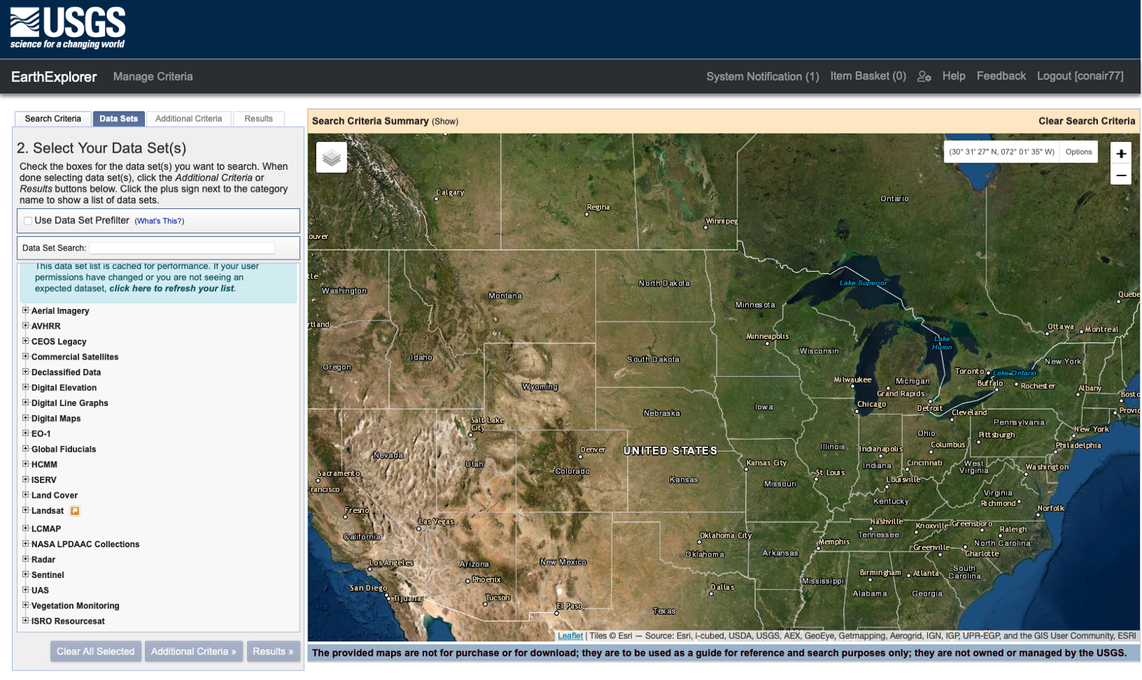
USGS’s EarthExplorer
After merging the two datasets I had the following features for each measured point:
-
Power Loss [dB] (Measured signal intensity power lost between the transmitter and receiver; This will be the model’s output prediction)
-
Signal Frequency [GHz] (The frequency of transmission)
-
Distance [km] (“As-the-crow-flies” distance between transmitter and receiver)
-
Height Difference [m] (Height difference between transmitter and receiver)
Feature Analysis:
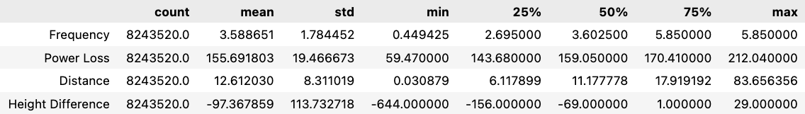
After completing the datasets, I moved to analyzing the data’s features. After dropping approximately 1000 N/A’s there are 8,243,520 complete rows. Leveraging pandas’ built-in .describe() function reveals the following:
Simple, but a few insights can be drawn:
-
Distance ranges from 0.03–80 km, but 75% of measurements are within 20 km. The algorithm will likely be better for short range measurements.
-
Height difference is usually negative, which makes sense. The Ofcom transmitter was elevated on a raised surface.
-
There is a high level of variability between feature magnitude. Normalization the data prior to training will be important.
-
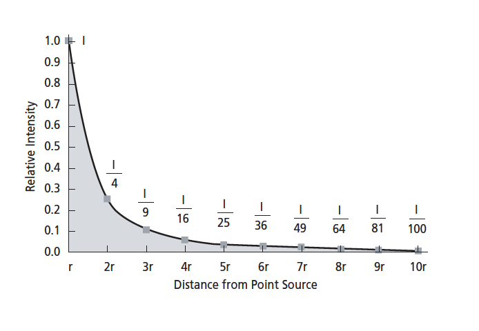
Finally, Power Loss starts low (59.47 dB), rapidly increases, and then flattens out. This matches what would be expected based on the inverse square law:
Seaborn’s pairplot() function plots every feature against the others, helpful for revealing correlation between features.
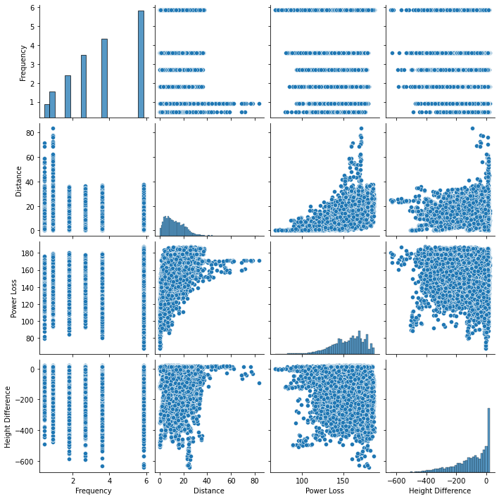
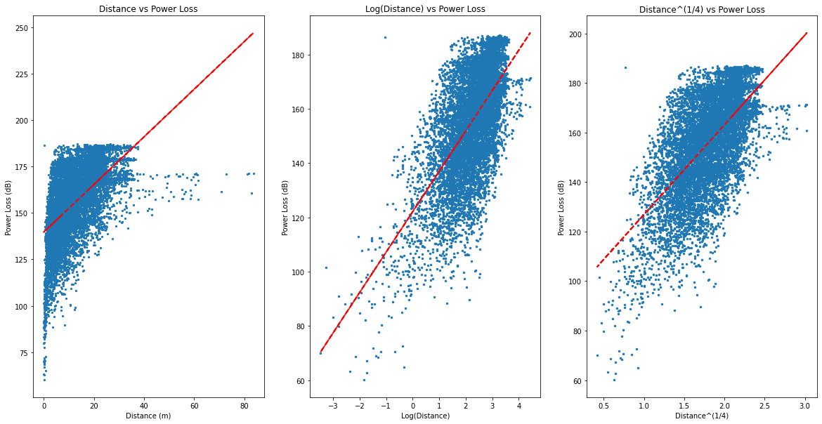
As expected, distance is clearly correlated with Power Loss, albeit not in a linear manner. The relationship is linearized by using a log or fractional power of distance.
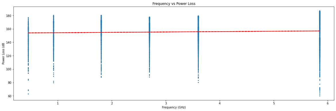
However, most features (such as transmission frequency vs power loss) do not show clear relationships:
Model Training:
Based on the available data and goals for the algorithm, a number of model architectures can be ruled out from testing. The model output will be a continuous value (the signal loss at a particular point), which rules out categorical prediction models such as logistic regression.
One model architecture that at first inspection seems promising is a Convolutional Neural Net (CNN). CNN’s classically excel on spacial data (typically images) and work well with continuous values. However, despite a dataset with a large number of measurements, it only contains 42 total “images” (7 cities at 6 different frequencies). Lack of data can sometimes be addressed by utilizing Transfer Learning, which involves taking a model trained on a large dataset of similar data and then training the final layer on the small real dataset. I was unable to find a quality model trained on radio frequency data, thereby eliminating CNN’s from testing.
In the end I elected to test 3 types of model architectures: Linear Regression, Boosted Tree Ensembles, and a Multilayer Perceptron Neural Net.
Splitting Data (Train, Cross-Validate, Test)
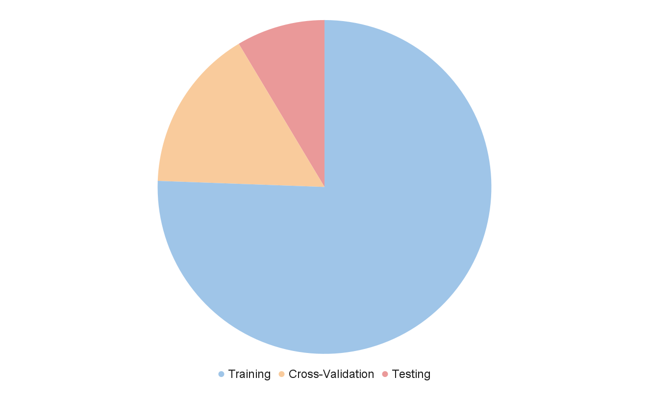
Before beginning training, I split the data into three subsets: Training, cross-validation, and testing. As its name suggests, the training dataset will be used for model training. The Cross-Validation dataset will be used for model performance evaluation and hyperparameter tuning. The test set will be used for final accuracy reporting.
Typically, random selection is used to partition the data. However, in this case due to the fact that the same cities are repeated for different frequencies, random selection may not be optimal. Models with larger numbers of parameters may “learn” specific cities’ layout between frequencies and become overfit. To avoid this, I selected one city (with its six frequencies) for cross validation, one for testing, and the remaining five for training.
I chose two medium sized cities for the smaller sets: Merthyr for cross validation and Stevenage for testing. On a per-measurement basis the data split was: Training: 75.58%, Cross-Validation: 15.83%, Testing: 8.59%
Boosted Tree Ensembles
Boosted Tree Ensembles are fairly distinct from the other two model architectures, so I started there. I used XGBoost (eXtreme Gradient Boosting) an open source implementation for building my model. It has proven to be highly competitive in ML competitions such as those hosted by Kaggle and has training times orders of magnitude faster than traditional ML architectures. A non-customized model also requires almost no code, as can be seen below:
This first TreeEnsemble achieved a Mean Average Error (MAE) of 10.26 dB, a strong improvement over FSPL’s MAE of 33.2 dB on the same dataset!
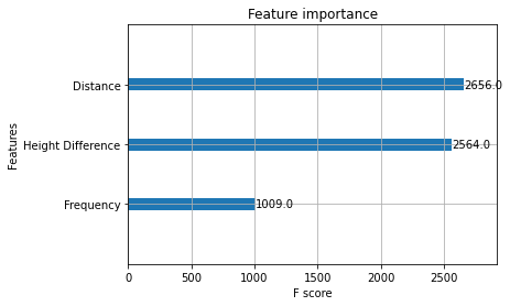
Tree Ensembles also allow for an additional interesting piece of feature analysis. By calculating the amount of improvement at each attribute split point and multiplying by the number of observations that node is responsible for results in a “Feature Importance” score. Below is the feature importance plot for the boosted tree implementation where, as expected, distance is the most important feature followed closely by height difference.
Multivariate Regression
The original ML architecture, Linear Regression is a good next step for evaluation. I used TensorFlow and Keras for both the linear regression and Neural Net architectures. Despite specializing in Deep Neural Nets, TensorFlow and its well-built out library works well for simple regression. I used the Keras API and layer terminology despite it not really applying to this simple regression example.
The initial regression model uses the features described in the data section, and has two “layers”. The first is simply a pre-processing normalization layer. The second is a single perceptron unit. The cross-validation dataset is used for the validation_data.
Below is the learning curve for the initial regression model, along with the error of the Free-Space Path Loss. Loss refers to the training set’s error, Val Loss refers to the cross-validation loss. Error corresponds to Mean Average Error (MAE).
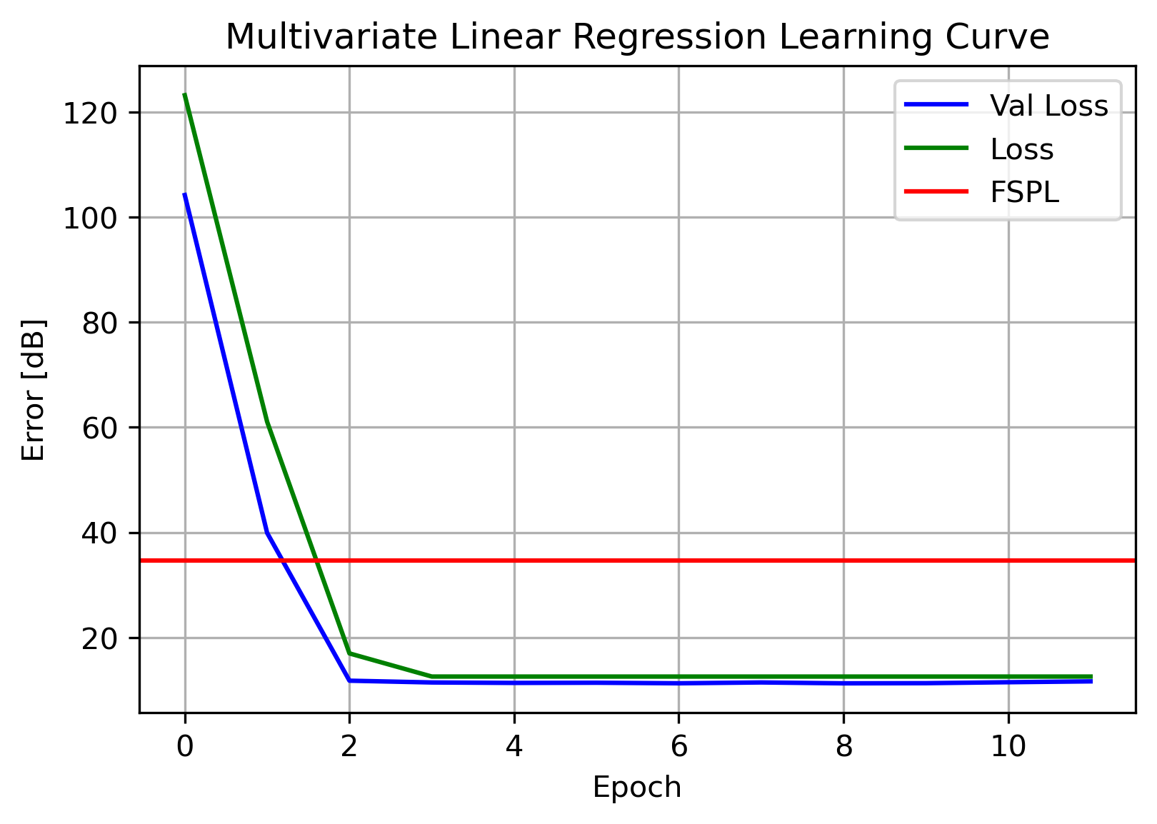
As can be seen above, the regression model strongly outperformed the FSPL model on the same data. FSPL had an MAE of 34.69 dB, and linear regression with 12.6 dB. Not as good as the Tree Ensemble, but not bad.
One of the main uses of a learning curve such as this is being able to see if the model has high variance or high bias (also known as overfit or under-fit, respectively). This is diagnosed by observing the training and validation losses over time.
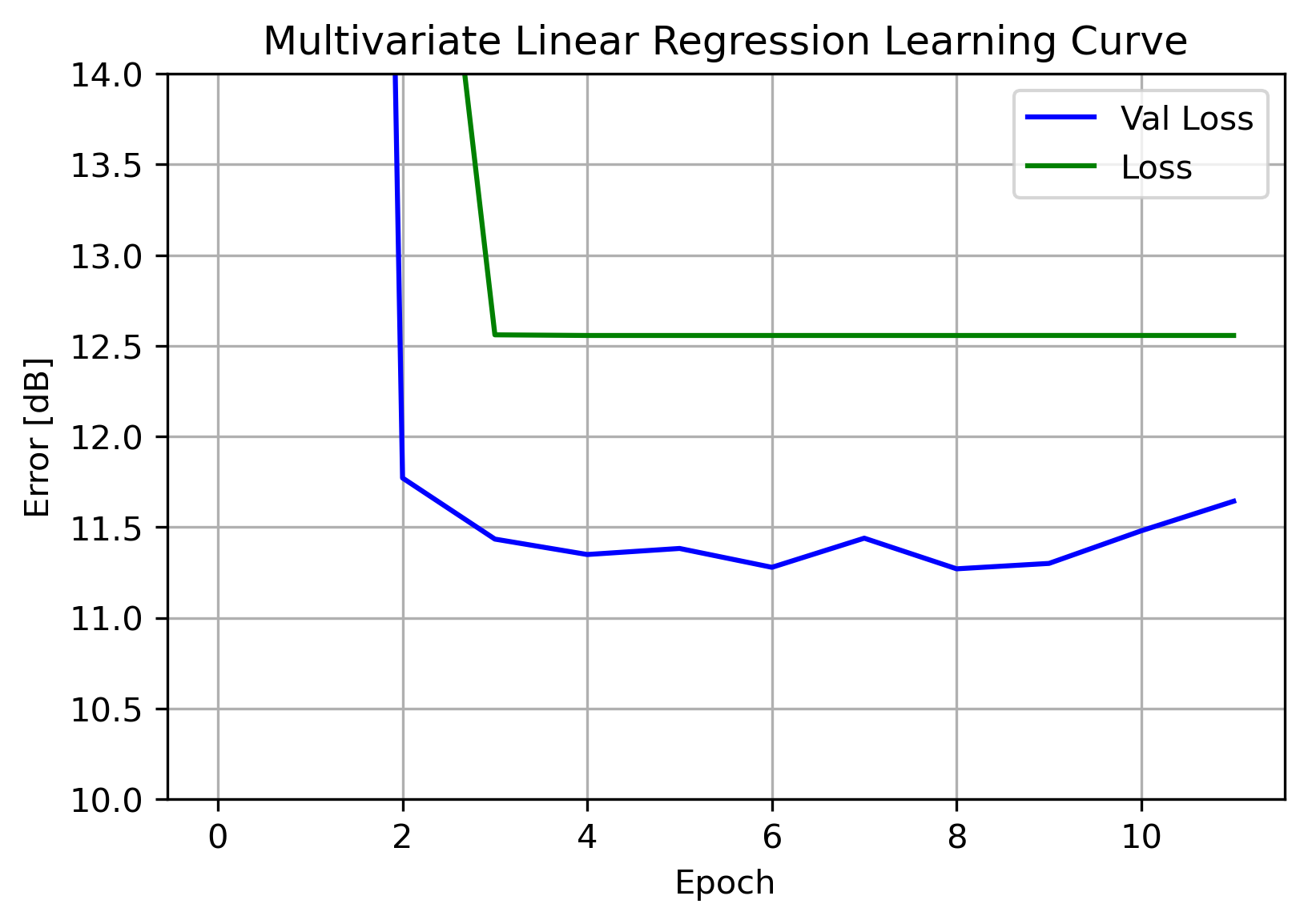
A callback was used to halt training after 5 epochs without improvement in the validation error. With both the training and validation losses remaining fairly flat, it can be concluded this model is not overfit nor under-fit. With no signs of overfitting, a Neural Net with a higher capacity for variance is a logical next step.
Neural Nets
The final type of architecture to evaluate was a Neural Net. Neural Net (NN) architectures learn their own features, often many times more than the original input features. This first, base NN is comprised of four layers : a preprocessing normalization layer, two hidden layers of 64 units, and an output layer with a single unit.
After compiling, the NN is fit and the learning curve plotted:
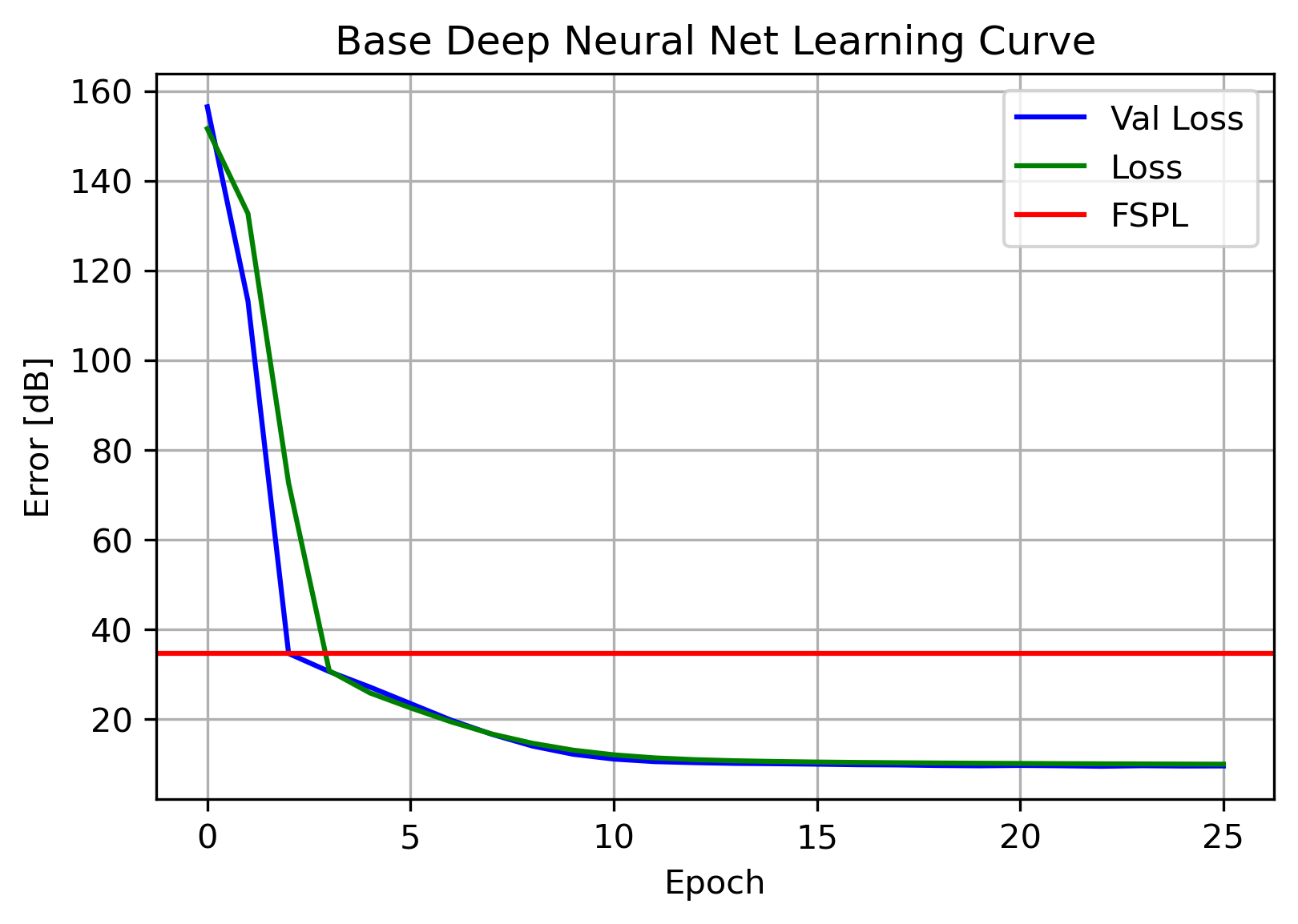
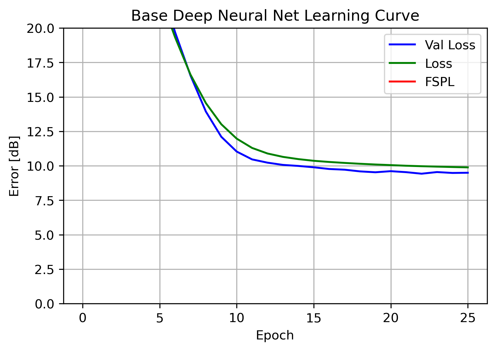
This NN was able to achieve a single-digit error level, beating out the Tree Ensemble! Again, similarly flat Loss and Validation Loss indicates a well-fit model, and implies an architecture with additional variance may lead to improvements. A parameter sweep can be leveraged to find an optimal architecture.
Neural Net Hyperparameter Tuning
The NN was the best performing model of the three, and by systematically varying two of the hyper-parameters batch_size and num_of_units it will hopefully reveal an even better performing model. Varying the number of units contained in each layer reveals the following:
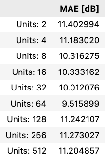
64 units was indeed the optimal number of units to use in each layer. Additional units simply appear to increase variance with no corresponding increase in accuracy. Moving on, a second grid sweep can be used to determine the optimal batch sizing as well:
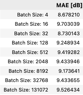
Using a batch size of 4 enables almost a full dB of error reduction. Moving to plotting the learning curve of this final model:
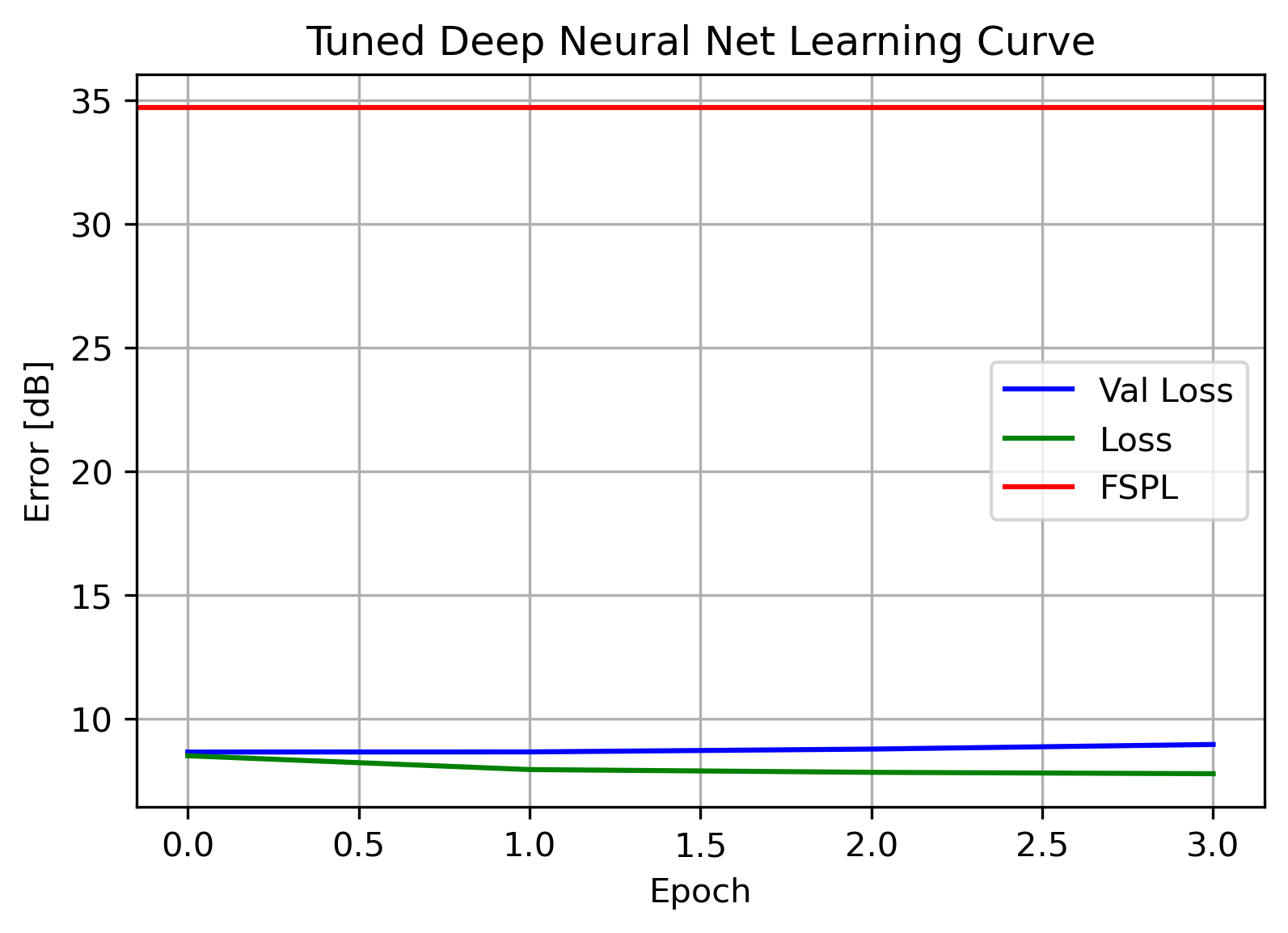
Again, with fairly flat learning curves, there does not appear to be signs of over or under fitting. This will serve as our production model.
ML Model Results:
After completing the survey of the three models above, these are the results:
The Tuned DNN had the best performance of the architectures evaluated, and will be the model selected to move forward with development. With model development complete, final accuracy can be reported using the yet-unseen test dataset: 11.24 dB
Export Model:
In order to run the model in an iOS environment, it needs to be converted to a type recognized by CoreML: Apple’s on-device ML Framework. CoreML requires that any ML model be stored in a .mlproject file. Luckily, Apple provides a Python package coremltools to assist in this conversion. After an import and a few lines of code, the model has been converted. It can simply be dragged and dropped into Xcode and be used to predict power loss!
Next Steps: Building the Mobile App
Check out the companion article here to see the process of building an iOS app capable of performing signal propagation modeling on-device.